This synthetic dataset consists of a single survey with a single loop consisting of 5 stations, 11 relative-gravity observations, and no absolute-gravity observations. In GSadjust terminology, in which "loop" refers to all of the observations for which a single drift correction is applied, the loop consists of two visits to each station, with the first station visited 3 times. The station order is 1-2-3-4-5-1-2-3-4-5-1.
Import data
Select "Load raw Burris data..." from the File menu. Open Test1.txt in the test_data/synthetic directory. Loop 0 is created.
In this synthetic example, there is only a single "observation" at each station. Therefore, the plots on the data tab show only a single point instead of a time series. Each station name can be selected in the tree view to show the associated data on the Data tab.
Note that the "Update adjustment" status indicator in the bottom right is highlighted, indicating the adjustment have not yet been performed:
Apply drift correction
Switch to the Drift tab by clicking "Drift". GSadjust displays a time series of the drift, with one line per station, starting at 0 for each station (see Drift tab for details).
In this example, drift is initially negative, as indicated by downward-sloping lines, but gradually becomes positive, as indicated by upward-sloping lines.
Four options are available for drift correction. The "None" and "Network adjustment" options do not change the plot. Selecting the "Roman" option updates the plot with vertical dashed lines to show the delta-g's, and a new table is shown in the bottom right with the average delta-g's. The "Continuous model" option displays an additional plot that shows the drift rate over time.
For now, proceed with the "Continuous model" option. Select "1st order polynomial" for the drift model type and "Constant" for the behavior at start/end.
Populate delta table
Switch to the Network Adjustment tab. From the Adjustment menu, select "Populate delta table - all surveys" (because there is only one survey and one loop, the other Populate... options will have the same effect). The delta-g's from the Drift tab are copied to the table on the Network Adjustment tab.
Add datum observation
For this simple example, there are no absolute-gravity observations. Instead, an arbitrary datum is applied to one of the stations.
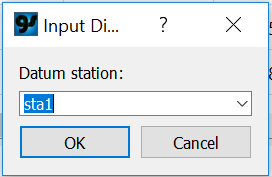
From the Adjustment menu, select "Add datum observation..." A dialog appears with a drop-down list of stations:
Select "OK" to select the default, sta1 (any other station is also acceptable, but will produce different results).
An arbitrary gravity value and standard deviation, 50,000 +/- 5 µGal, is applied to sta1 and shown in the datum observations table. This value can be changed by double-clicking it in the datum observations table, as can the standard deviation, measurement height, and gradient. The datum date is an arbitrary string and has no effect on the results.
Perform adjustment
From the adjustment menu, select "Adjust current survey" (because there is only one survey, "Adjust all surveys" will have the same effect). Alternatively, click the button on the tree view toolbar, or use the keyboard shortcut Ctrl+2. The adjustment will proceed using the default Numpy method.
Adjustment results (a single, best-fit gravity value at each station) are shown in the adjusted station values table at the upper right. Adjustment statistics are shown in the table at the lower right. Note that the Chi-test was accepted, and the a posteriori standard deviation is near one. These indicate the adjustment was acceptable. The a posteriori standard deviation less than one indicates that the estimated standard deviation of the observations was higher than the adjustment results indicate. The delta-g standard deviations can be automatically scaled using the "Scale std. dev. from results" menu command or the corresponding button on the Tree view toolbar. After doing so the "SD for adj." value shown on the delta-g table is lowered to 2.7 µGal, and the standard deviation a posteriori is 1.0
Note that the "Update adjustment" status indicator in the bottom right is no longer highlighted.
For this simple example, the tools for evaluating results are limited. A histogram of delta-g residuals ("Plot residual histogram", or Ctrl-H) is uninformative owing to the small number of observations. Because there is only one datum observation, the adjusted value matches the observed value exactly and the "Plot adjusted datum vs. measured" plots only a single value of zero.
Export results
From the Tools menu, select "Write tabular data". A comma-separated value (.csv) file with the filename "GSadjust_TabularData_..." followed by the date is written to disk with the values shown in the adjusted station values table. Optionally, the results table can be highlighted by clicking in the upper-leftmost cell, then right-clicking and selecting Copy to clipboard. Data can be pasted into Excel or a text file.
From the Tools menu, select "Write metadata text". A text file (.txt) with the filename "GSadjust_MetadataText_..." is written to disk with a narrative summary of the adjustment. This text can be used in a metadata file.
From the Tools menu, select "Write adjustment summary". A text file (.txt) with the filename "GSadjust_Summary_..." is written to disk showing the observations used in the adjustment and the results of the adjustment. This file includes all of the information necessary to re-create the adjustment results.
Save the workspace
To facilitate future re-processing or evaluation, the workspace should be saved by selecting "Save workspace as..." from the File menu. A file save dialog is shown; save with an appropriate filename. A ".gsa" extension is added if not specified. The workspace is written to file in JSON format. This file can be re-loaded into GSadjust using the "Open workspace..." command on the File menu. It should not be edited outside of GSadjust.