This real-world dataset includes 38 stations and 8 absolute-gravity measurements. Two surveys were carried out, each with two relative-gravity meters.
Two saved workspaces are provided. The file gsadjust\test_data\field\Burris\complete_workspace1.gsa is worked through step 4 below (Earth tide correction). The file gsadjust\test_data\field\Burris\complete_workspace2.gsa is worked through step 7 below. These files can be loaded to skip ahead in the tutorial.
1. Import relative-gravity data
First,
load data from the first meter (serial number B44) used on the first survey. Select "Load raw Burris data..." from the File menu. Open B44_2017-12-05.txt in the test_data/field/Burris directory. Survey 2017-12-05 and Loop 0 are created and selected.
In this real-world example, each station occupation consists of several samples. The gravity time series (and feedback, tilt correction, and Earth tide correction time series) are shown in the table and plots on the Data tab. The respective data for each station can be shown by selecting the station in the left-side tree view.
Next, load data from the second meter (B108) used on the first survey. Select "Append loop to current survey..." from the File menu. Open B108_2017-12-05.txt in the test_data/field/Burris directory. A dialog appears to select the meter type; choose "Burris". Loop 1 is created but not selected. Double-clicking "1" will update the contents of the Drift tab.
Load the data from the second survey in a similar manner. First, add the data from meter B44 (B44_2018-02-27.txt) using "Append survey to campaign...". A dialog appears to select the meter type; choose "Burris". Survey 2018-02-27 and Loop 0 are created but not selected (you may need to click the "expand" arrow next to the survey name to show the loops). Double-click Survey 2018-02-27 to select it. Finally, append the data from meter B108 (B108_2018-02-27.txt) using "Append loop to current survey...". A dialog appears to select the meter type; choose "Burris". Loop 1 is created but not selected.
The samples collected at each station occupation are displayed on the table and plots on the Data tab:
For now, don't worry about which samples are included at each station (controlled by the check boxes in the table). These can be fine-tuned after successful adjustment results are obtained.
2. Edit data
Two items need correcting in the raw data before loading: two stations were collected on the wrong dial setting, and one station must be duplicated so it can be included in two different loops.
The stations collected with the wrong dial setting are obvious from the drift plot. With the Drift tab displayed, double click 2018-02-27 Loop 1 to select it (data from meter B108). Note in the drift plot the very large step in the drift:
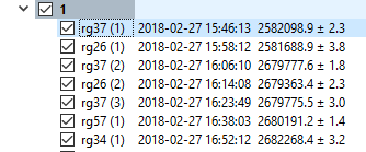
This is caused by an incorrect dial setting for the first two stations. Its also apparent by the large difference in gravity for the first two occupations at rg37 and rg26 in the data tree view:
In this case, these first two station occupations should be deleted. Select them (with rg37 highlighted, hold down the shift key and click rg26) and right-click to bring up the
context menu. Select Delete station(s). The drift plot is updated.
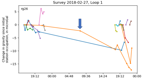
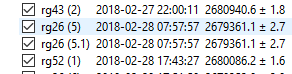
Now, on the updated drift plot, note the single occupation at station rg26 in the center of the survey, at about 8:00 (click on the orange line to show the station):
This happens in the common situation when the last station of the day is observed as the first station the following day. Station rg26 was occupied last on 2018-02-27, and first on 2018-02-28. The point on the plot represents the average time midway between these occupations. To see this, display the Data tab and select the rg26 occupation at 7:57:
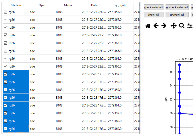
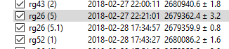
First, we'll duplicate rg26 by right-clicking and selecting Duplicate station. Now there are two identical rg26 occupations in the data tree view:
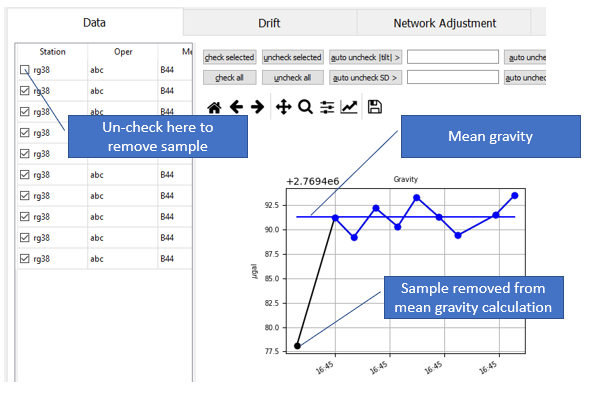
Select the first one, "rg26 (5)". With the Data tab displayed, select (by shift-clicking) all of the samples on 2018-02-28:
Next, click the "uncheck selected" button at right. The plot and mean gravity value are updated. In this example, the two occupations have very similar gravity values but that is not always the case. Repeat with the "rg25 (5.1)" occupation, unchecking the samples from 2018-02-27. The contents of the tree view are updated to reflect the checked samples:
Now, on the Drift tab, the central point has been replaced by two points on 2017-02-27 and 2018-02-28.
3. Organize data
Next, each loop needs to be
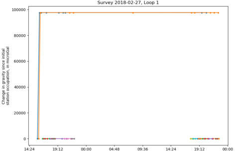
subdivided into smaller loops. Viewing the Drift tab shows a long gap in the data for each of the surveys (double-click the loop name to show drift for that loop).
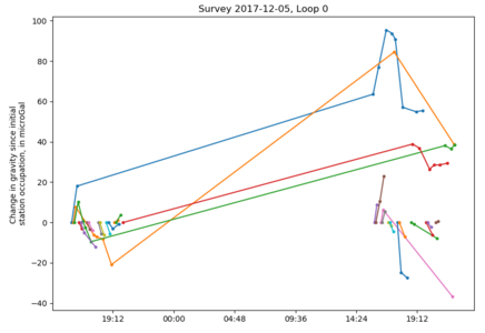
For example, Survey 2017-12-05 Loop 0 shows two groups of data separated by an overnight period without data:
Because these two periods, representing two consecutive days of field work, have unique drift behavior, they should be divided into separate loops (a loop denotes the group of stations for which a single drift correction is applied). The loops can be separated in one of two ways. Generally the easiest is to apply a time-based threshold, by which gaps in data greater than a specified value are moved to a new loop. Do this using the "Divide selected loop..." option on the Edit menu. A dialog is shown where the time threshold can be specified; the default value of 8 hours works well to divide surveys on successive days.
After clicking OK in the threshold dialog, a new loop (Loop 2) is created under the 2017-12-05 survey. Select each loop in the 2017-12-05 survey (by double-clicking the loop name) with the Drift tab visible to see how the new loops were created
An alternate way to divide loops is to select the stations in the tree view (by shift-clicking or dragging across a group of stations) to be moved to a new loop and selecting the "Move station(s) to new loop" command on the
right--click context menu.
Divide all of the remaining loops using the same time-based threshold. Before dividing, each loop must be selected by double-clicking the loop name.
4. Update tide correction
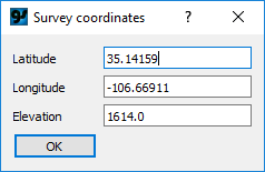
Although the Burris relative-gravity meter (and Scintrex meters) apply a tide correction, for this study the Agnew model provides a more accurate correction. To
update the tide corrections, from the Edit menu select Tide correction, then choose the "Agnew" option. A dialog is displayed to enter coordinates:
The dialog is pre-populated with the mean latitude and mean longitude of the observations. After selecting OK, the meter-supplied tide correction is removed and the new tide correction applied. To revert to the meter-supplied tide correction, select Tide correction from the Edit menu, then "Meter-supplied".
Note that the Agnew tide correction is reported to 0.1 µGal, compared to the Burris internal tide correction which is reported to 1 µGal.
5. Apply drift correction
Next, click on the
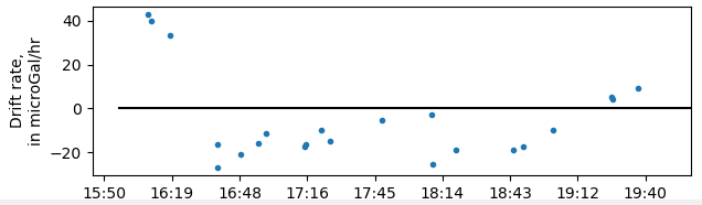
Drift tab. The plot title should show Survey 2017-12-05, Loop 0. If a different survey is shown, double-click "0" under the 2017-12-05 survey to select Loop 0:
The drift plot shows a short period of positive drift (upward-sloping lines) followed by generally negative drift (downward-sloping lines). This change in drift rate is visible when when the "Continuous model" drift correction method is
selected:
For now, select the Roman drift correction method. The plot is updated with vertical dashed lines to indicate how the gravity differences (delta-g's) are calculated. The Roman method is a good all-purpose method that accommodates periods of inconsistent drift.
Also apply the Roman drift correction method to the remaining loops by double-clicking each loop in turn and selecting the Roman method.
6. Populate delta table
Next, show the
Network Adjustment tab, which should be empty. First we want to copy the gravity differences (delta-g's) from the Drift tab to the Network Adjustment tab. When the delta-g's are copied, they retain their link to the data in the tree view, but not to the delta-g's on the Drift tab. That is, if the gravity value at a station occupation changes (for example, if samples are unchecked on the Data tab), the delta-g(s) that include those stations are automatically updated on the Network Adjustment tab. Any changes on the Drift tab (for example, changing the drift correction method) are not reflected on the Network Adjustment tab until the delta table is
updated.
To populate the delta table for all surveys, select the "Populate delta table - all surveys" command on the Adjustment menu. Later, when iteratively updating the observations used in the adjustment (for example, testing a single loop), the other "Populate delta table" commands are useful.
7. Import datum observations
The
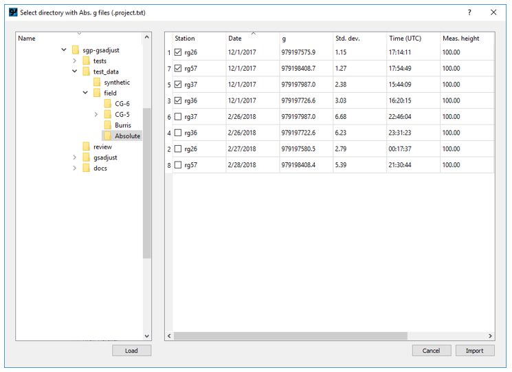
datum observations can be absolute-gravity measurements stored in *.project.txt files generated by 'g' software used with Micro-g Lacoste absolute-gravity meters. First, make sure the 2017-12-05 survey is selected (if not, double-click on it to select). Select "Import abs. g from project files..." from the Adjustment menu. In the dialog, navigate to the gsadjust\test_data\field\absolute directory. Click the "Load" button at bottom left. The relevant details from the .project.txt files in the absolute directory are shown:
Sort by Date (click on the column header), then check the 4 observations from 2017-12-01. Click import and the observations will appear on the datum table.
Select the 2018-02-28 survey and import the absolute-gravity observations from February 2018.
Shortcut: The saved workspace complete_example2.gsa is saved at this point.
8. Perform adjustment
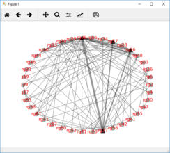
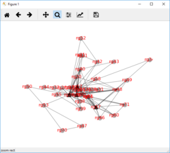
Now, sufficient data are present to perform the network adjustment. Network graphs can be viewed in circular or map-view layout using the two commands on the Tools menu:
|
Tools menu > Network graph - circular
|
|
Tools menu > Network graph - map view
|
|
|
|
|
In the network graphs datum (or absolute-gravity) stations are shown as black triangles and relative-only stations are shown as red circles.
To perform the network adjustment, select "Adjust all surveys" from the Adjustment menu, or click the corresponding button on the tree-view toolbar:

. The Adjusted station values and Least-squares statistics tables on the Network Adjustment tab will update. These tables are unique to each Survey; by changing the selected survey (double-clicking in the tree view) the tables will update.
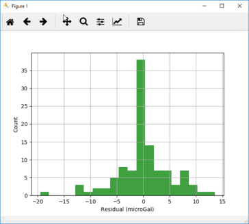
View the adjustment residuals using the "Plot residual histogram command" on the Adjustment menu (close the network graph window first if it is still open):
9. Change adjustment options
Although the network adjustment was successful and results were obtained, note in the statistics window (bottom right) that the Chi-test was rejected for both surveys and the "SD a posteriori" statistic is greater than 1, meaning that the uncertainty (standard deviation) of the input observations was underestimated (that is, the observations don't fit together as well as the measurement uncertainty suggests). Several steps can improve the results:
First, note that the standard deviation of many of the delta-g's is very low (sort the Relative-gravity differences table by clicking on the "Residual" column heading). The standard deviation will be zero when using the Roman drift correction method if only one delta-g exists between a particular station pair. Low standard deviations cause these measurements to be matched nearly exactly (residuals are close to zero), while measurements with high standard deviation are weighted much less.
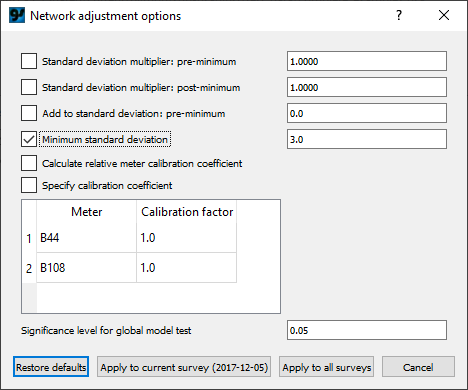
When surveying with relative-gravity meters, there is a practical lower limit on how accurately delta-g's can be observed. The delta-g uncertainty includes the uncertainty from both station occupations, uncertainty from the drift corrections, and uncertainty from unaccounted tares. A minimum lower limit for delta-g standard deviation can be specified in the
Adjustment options dialog on the Adjustment menu:
Check the box next to "Minimum standard deviation", keep the default value of 3.0, and click "Apply to all surveys". Now in the Relative-gravity differences table the "SD for adj." column shows the larger of 3 or the uncertainty determined from the drift adjustment. Note that the input data for the adjustment has changed and the adjustment results are now outdated, as shown by the status indicator in the bottom right:
Repeat the adjustment (
) to update results and clear the status indicator.
10. Update drift correction
After the adjustment the Chi-test was still rejected for the 2017-12-05 survey, but accepted for the 2018-02-27 survey. While viewing the 2017-12-05 survey on the network adjustment tab, note that several of the residuals are fairly large: less than -10 or greater than 10. Sorting the Relative-gravity differences table by Loop shows that most of the large residuals are associated with Loop 2. Double-click on loop 2 to select it and display the Drift tab:
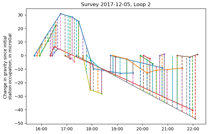
Note the two long segments (red and grey) that stretch across nearly the entire survey, corresponding to stations rg30 and rg26 (click the line to show the station name at the top left of the plot). Using the Roman method, relative-gravity differences are calculated between these two stations and nearly every other station, with the drift rate interpolated over the 5+ hour period between repeat occupations. Based on repeat occupations at the other stations, it appears during this 5+ hour period there was only a short period of high drift (around 17:30 to 18:00), or possibly a tare, and much lower drift during the remainder of the period.
To remove this spurious drift estimate, a maximum time threshold between stations can be specified by checking the box to the right:
Now, any station occupations separated by the specified threshold will be ignored in the drift calculation (for either the Roman or Continuous drift-correction options).
The delta-g's on the Network Adjustment tab are automatically updated.
Repeat the adjustment (
) to update results and clear the status indicator. Now the Chi-test is accepted for both surveys and the SD a posteriori statistic is close to 1, indicating the standard deviation estimated from the observations is close to the standard deviation estimated by the network adjustment.
12. Fine-tune the individual station values
Next, the estimate of the average gravity reading at each station occupation can be improved by deactivating samples as needed. With the Data tab displayed. go through each station in the left-hand tree view and deselect samples as needed by unchecking them in the table on the Data tab. For example, with the Burris meter often the first 1 or 2 readings appear to be outliers:
As samples are checked or unchecked, changing the mean gravity value, the gravity differences on the Drift tab and the Network adjustment tab are updated automatically. However, the network is not automatically re-adjusted.
13. Update adjustment results
Once final station values are determined, appropriate drift corrections made for each loop, and an initial adjustment performed, the standard deviations should be scaled so that the standard deviation a posteriori statistic is close to one. This can be accomplished by the "Scale std. dev. from results" command on the Adjustment menu, or the

button on the
Tree View toolbar. This scales the standard deviation of each delta-g ("SD for adj." column in the
relative-gravity differences table). See the
network adjustment options page for more information about how the scaling is applied.
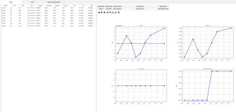
14. Calculate gravity change over time
If more than one survey exists, the change in gravity over time can be calculated with the
Compute gravity change command on the Tools menu. This shows a table of gravity change over time in the first n-1 columns, and cumulative change in gravity since the first survey in the next n-1 columns (where n is the number of surveys). If a station is not present in a survey the null value -999 is shown.
Three options are available for further analysis. First, a time-series of gravity change relative to the first observation at each station can be shown by clicking the Plot button in the gravity change table. Second, if station coordinates are available, a map view of gravity change can be shown by clicking the Map button. Finally, a more complete table of results which includes gravity values, uncertainties, coordinates, and gravity change converted to meters of water using the 1-d horizontal-infinite slab approximation (41.9 µGal = 1 m of free-standing water) can be shown by clicking the Show full table button.
15. Export results
Finally, results can be
exported in several ways:
1) The adjusted station values on the network adjustment tab can be highlighted (clicking the upper left corner highlights all cells), copied by right-clicking on the table, and pasted into Excel or a text file as tab-delimited data. Similarly, results can be copied and pasted from the
gravity change table.
2) Adjusted station values can be exported to a comma-delimited text file using Write tabular data on the Tools menu.
3) A narrative summary of the adjustment, including statistics and the number of observations, can be written to a text file using
Write metadata text on the Tools command. The resultant text is suitable for describing the data-processing steps in a metadata file to accompany the adjustment results.
4) A complete list of all data used in the adjustment can be written to a text file using Write adjustment summary on the Tools menu.